Looking at one token of LLM inference
I wanted a way to see exactly what happens when a language model produces one token, and how much of that work can actually run at the same time. The usual mental model is "a big stack of matrix multiplies," which is true but hides most of what matters for latency: which steps have to wait on which, what data each step reads, and what has to be kept around for the next token. So I built an interactive visualizer that draws one decode step as a dependency graph and then counts and schedules every operation in it.
Open the visualizer · two views, Token pipeline and Token statistics, with a model selector in the corner.
The goal
The question I was after is the serial versus parallel capacity of inference on a per-token basis. A GPU (or any accelerator) is extremely wide, but a single generated token has a long chain of steps that can't start until the previous one finishes. I wanted to break that chain down into its actual operation types, sort the data each operation touches into three lifetimes, and measure two things directly: how deep the chain is, and how wide it ever gets.
The three data lifetimes ended up being the most useful way to look at it:
- Static (blue): weights, norm scales, RoPE coefficients. Read-only during inference; the same bytes serve every token.
- Ephemeral (green): activations produced and consumed within this one token, such as projections, scores and gate values. Gone when the token is done.
- Mutable state (red): the attention K/V cache, the linear-attention recurrent state and the short convolution buffer. Read and then written every token, and carried forward to the next one.
Once every value has one of those colors, I classify the operation that combines them by its operands instead of by its arithmetic symbol. W × x with a static W is a fixed linear transform: the coefficients are known ahead of time and could be stored, cached or streamed. q · k looks like the same multiply-accumulate, but both sides were produced at runtime, so none of it can be precomputed. You can't see that difference in a FLOP count, and it matters a lot for where the work can live.
What it models
The diagrams cover three Qwen hybrid decoders with pinned configurations: a 2.4T-parameter mixture-of-experts model (95B active, 512 experts with 10 selected plus one shared), a dense 27B with 4-bit weights, and a dense 0.8B. All three interleave three Gated DeltaNet blocks (a linear-attention layer with a fixed-size recurrent state) with one full-attention block. The scenario is always one new token after one million cached positions, which makes the cost of history easy to see. That's past the models' configured 262K context, so treat it as a sizing scenario and not something you'd actually run.
Token pipeline view
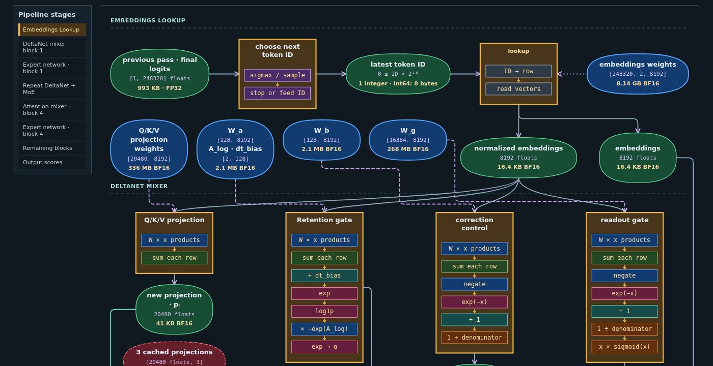
The first view is the dependency graph for a single token, laid out top to bottom through the embedding lookup, a DeltaNet block, the expert network, an attention block and the output scores. The remaining blocks repeat the same pattern. Rounded bubbles are data, colored by lifetime and labeled with shape and byte size. The gold boxes are transforms, and each one is split into its ordered internal sub-blocks: a projection is "products, then sum each row"; a sigmoid gate is "negate, exp, +1, reciprocal, multiply". Each sub-block is colored by its operation class: fixed linear (static coefficients), dynamic multiply/divide (both operands live), add/subtract, reduction, nonlinear transfer (exp, log1p, rsqrt), position-selected (RoPE), compare/select (top-k, argmax, sampling) and route/store (lookups, cache appends, fanout).
Clicking a node opens a detail panel with its equation, its actual inputs and outputs in the graph, what work inside it is parallel, and what it has to wait for. Below the graph there's a ledger of what each block saves for the next token. On the 2.4T model, each DeltaNet layer updates an 8.39 MB FP32 state in place and never grows, while each attention layer appends 4.1 KB of K/V per token on top of 4.1 GB already cached at a million positions.
Token statistics view
The second view takes the same graph and turns it into numbers. The part I care about most is the schedule. Every sub-block drawn in the pipeline counts as one operation taking one unit of time, regardless of its tensor size, and the whole token is expanded across all blocks and scheduled as early as its dependencies allow. Matrix rows, heads, coordinates and the ten routed experts don't add to the count; they're the width inside an operation. What's left is the shape of the dependency chain itself.
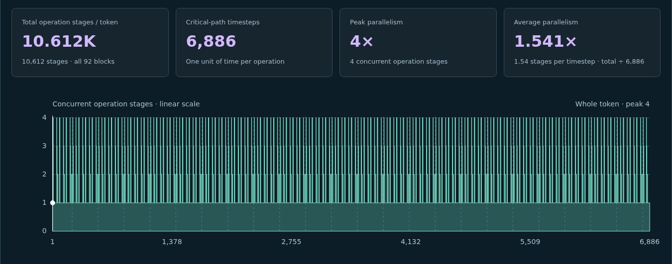
The numbers came out pretty lopsided:
- 2.4T MoE: 10,612 operations per token, a critical path of 6,886 timesteps, peak parallelism 4, average 1.54.
- 27B dense: 5,337 operations, critical path 3,897, peak 4, average 1.37.
- 0.8B dense: 2,001 operations, critical path 1,467, peak 4, average 1.36.
So at the level of whole operations, decoding one token is almost entirely serial. The widest it ever gets is the four-way fan-out at the start of each mixer (the separate projections for Q/K/V, the gates and the correction terms), which narrows back to one as those branches join. Zooming into a single block shows the pattern pretty clearly:
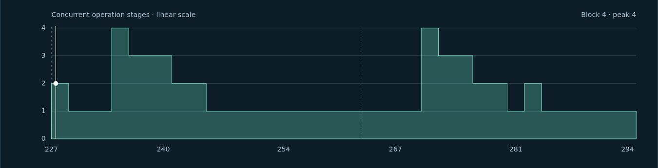
All of the real parallelism is inside operations: thousands of rows in a projection, dozens of heads, ten experts at once. Basically none of it is between them. That's why single-stream latency comes down to depth times per-operation latency more than peak FLOPs, and why the things that help are the ones that add more independent work per step (batching, speculative decoding) or make each of those ~7,000 steps faster.
Where the work and bytes go
The rest of the statistics view is a ledger of math and data movement for the same token. For the 2.4T model at a million positions, that's about 847 billion multiply-accumulates (≈1.69 TFLOPs), plus 1.47 billion exponentials. 99.6% of those exponentials are attention softmax over the cached history; everything else in the model needs only about 5 million.
The bandwidth table assumes an ideal streaming pass that reads each active weight and each shared K/V element once. On the 2.4T model that's 282 GB per token, or 28 TB/s at 100 tokens/s. About two thirds of that is static weights (186 GB, only the selected experts) and one third is K/V (94 GB). The smaller models flip that split. On the 4-bit 27B, K/V reads are 83% of the 79 GB per token, and on the 0.8B they're 89%. So at long context, mutable state ends up being a bigger bottleneck than the static weights. The DeltaNet layers are the exception: their recurrent state stays the same size no matter how long the history gets, so they're less than half a percent of traffic.
There's also a dependency graph between operation types, weighted by how many values each type hands to the next. I see it as a starting point for thinking about which operations want to sit next to each other. The operation breakdown table lists every stage with its count and pipeline position.
Caveats
This models the math logically; it doesn't simulate hardware. "One unit of time per operation" is crude on purpose: an exp over 8,192 values and a matrix product over 8,192 × 20,480 don't cost the same, and real kernels fuse a lot of these stages together. What I wanted to show is the dependency structure, which you can't remove by adding more hardware width. The counts come from the published configurations and reference implementations. The 4-bit profile leaves out quantization metadata, and nothing here accounts for tiling, cache residency or activation spills.
It's plain JavaScript and SVG without a framework, and everything is computed in the browser from the model dimensions. Switching models rebuilds both views.