How much analog noise can a small LLM take?
Ryle ·
Analog and optical inference hardware computes with physical signals, and physical signals are noisy. Every analog multiply, every stored value and every readout comes back a little off, and usually differently off each time. Before designing anything along those lines I wanted to know how much noise a language model actually tolerates and which parts of it are sensitive. So I took a small open model, Qwen3.5-0.8B, injected controlled noise at each place an analog machine would touch it, and measured what happened on benchmarks and on long text.
In short: most of the model shrugged off 1% noise, and one part didn't. Noise on the recurrent state, the memory that some layers rewrite on every token, was a hundred times more damaging than the same noise anywhere else. And the usual short benchmarks almost completely missed it. At 1% error per state write, ARC-Easy and HellaSwag scores lost at most 5.7% relative to the clean model, while a retrieval test over a 4,096-token context fell from 12/12 to 4/12, which is about what you'd get by guessing.
The model and what it remembers
Qwen3.5-0.8B is a hybrid. Of its 24 layers, six are ordinary attention layers and 18 are Gated DeltaNet layers, a kind of linear attention. That matters here because the two kinds remember the past differently, and memory turned out to be the whole story.
An attention layer keeps a KV cache: for every token it has seen, it stores a key vector and a value vector, and each new token compares its query against all the stored keys. Each row is written once and then only read. A DeltaNet layer instead keeps a fixed-size recurrent state, here a 128×128 matrix per head, and on every token it decays that matrix slightly, applies a small correction from the new token and writes it back. DeltaNet layers also have a short convolution over the last four tokens' projected inputs, which needs its own little history buffer.
| Stored object | Values written per token | Values held at 4k context |
|---|---|---|
| Attention K/V cache (6 layers) | 6,144, appended | 25,165,824 |
| DeltaNet recurrent state (18 layers × 16 heads × 128 × 128) | 4,718,592, all rewritten | 4,718,592 |
| Convolution history (18 layers) | 110,592, appended | 331,776 (last three tokens) |
The KV cache grows with context, but each value in it is written once. The recurrent state stays the same size, but every value in it gets rewritten on every token, so 4,096 tokens means 4,096 noisy writes on top of each other. Which of those hurts more isn't obvious from the architecture, so I measured it. (I drew the same split between static, per-token and carried-forward data in an earlier visualizer of one decode step.)
Noise models that can be told apart
My first attempt was the obvious one: replace every operation in the model with a noisy version that modeled one particular hardware design, and score the result. It failed badly. One of the gentler configurations lost 19% on HellaSwag and a code-retrieval probe dropped from 8/8 to 3/8. But with dozens of noise sources switched on at once I couldn't tell which one was responsible, and every number depended on hardware assumptions I hadn't verified. The simulation code grew to about 70 Python scripts, most of them modeling specific hardware ideas that I'm leaving out here.
So I restarted with something more boring and more useful. The weights and the embedding table stay exactly as in the checkpoint, in FP32. Noise goes in at named interfaces, one family at a time, and every interface has an explicit lifetime: either the noise is fresh on each token, or it's written into something stored and every later token reads the same corrupted value.
The noise itself is simple. At an interface, the code takes groups of up to 128 adjacent values, computes their RMS (root mean square, the typical magnitude), and adds independent Gaussian noise with a standard deviation of that RMS times the amplitude. "1% RMS" means each group gets random error about 1% the size of its own signal. That's a deliberately abstract unit. It isn't a physical noise floor, and it hands the model a free automatic gain control that real hardware would have to pay for. But it puts every interface on the same scale, so the comparison is fair.
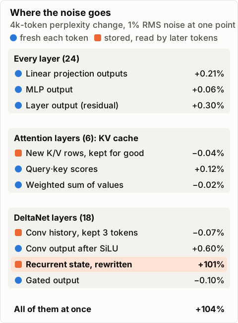
The numbers in that diagram are changes in perplexity on a 4,096-token block of WikiText. Perplexity measures how surprised the model is by the real next token, averaged over the text; lower is better, and the model sees the correct previous tokens at each step. It's a sensitive early warning, though not a measure of answer quality, which comes up again below.
To keep the noise honest, the DeltaNet recurrence runs in a plain Python loop, one token at a time. Noise has to land on every individual state write, and the next token has to read the actual noisy state, not a clean recomputation from the prompt. That rules out the fast fused kernels and makes long contexts slow. An ideal run with noise turned off has to reproduce the stock model's logits (within about 6 parts in a million) before any noisy result counts.
The sweep
Each interface was swept at 0.1%, 0.3%, 1%, 3% and 10% RMS, with extra points added where perplexity crossed a +10% marker. That marker was only used to decide where to sample more densely, not to pass or fail anything. The full screen was 13 noise families, plus controls for drift, fading and fixed per-cell errors.
| Interface (fresh noise) | 0.3% RMS | 1% RMS | 10% RMS |
|---|---|---|---|
| New K/V rows | −0.01% | −0.04% | +0.21% |
| Query·key scores | +0.03% | +0.12% | +5.9% |
| Weighted sum of values | −0.01% | −0.02% | +3.4% |
| Recurrent state write | +1.6% | +101% | +5,463,551% |
| Conv history write | −0.02% | −0.07% | +0.19% |
| Linear projection outputs | +0.02% | +0.21% | +30% |
| Conv output after SiLU | +0.14% | +0.60% | +60% |
| MLP output | +0.01% | +0.06% | +2.6% |
| Gated output | −0.03% | −0.10% | −0.51% |
| Layer output (residual) | +0.06% | +0.30% | +21% |
| All of the above at once | +1.8% | +104% | +4,487,317% |
Change in 4k perplexity, one interface at a time. Small negative values are noise in the measurement, not improvements.
Two things stand out. The KV cache is remarkably tolerant: 10% error on every stored key and value row barely registers. And the recurrent state is in a different league from everything else. It's already noticeable at 0.3% and doubles perplexity at 1%. The fresh activation interfaces sit in between and only start to matter somewhere between 3% and 10%.
Why the state is different
A DeltaNet update multiplies any error already in the state by α(I − βkkᵀ), where α is the learned decay (between 0 and 1), β is a learned write strength and k is the new token's normalized key. That factor never grows an error, so the recurrence isn't an explosive amplifier. But α is close to 1 in exactly the layers that need to remember a lot, and that means old errors shrink slowly while a new one arrives on every token. As a toy example, if each write adds noise with variance q and old error shrinks by a factor ρ per token, the error settles at q / (1 − ρ²). At ρ = 0.99 that's about 50 times the per-write variance, or 7 times the per-write RMS. The real model is messier than that, since noisy state also changes later keys and gates, but it gives the right intuition: layers built to hold information for a long time also hold noise for a long time.
A pulse test shows it directly. I injected a single 3% error at token 128 and nothing after it, then measured how far the model's predictions had drifted (as KL divergence, a measure of the difference between two probability distributions) 256 to 382 tokens later.
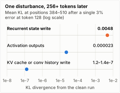
A fresh, exact embedding for every new token doesn't reset anything. The token's hidden vector is recomputed from scratch, but 18 of its 24 layers read a state that still carries every earlier error.
What I measured
I set the target before running anything: strictly less than 10% relative score loss against the clean original model, on standard benchmarks, with each task and metric judged separately. Relative means a task the clean model gets 80% right needs at least 72%.
- ARC-Easy: grade-school science multiple choice.
- HellaSwag: pick the most plausible ending for a short everyday scene, out of four.
Both are scored with EleutherAI's lm-evaluation-harness (0.4.13), which compares the model's likelihood of each answer instead of parsing generated text. It reports acc and acc_norm, where acc_norm divides by answer length so long answers aren't penalized. I kept all four numbers separate and didn't average them.
On top of that, three long-context diagnostics. Perplexity, KL and next-token agreement on fresh 4,096-token WikiText. Twelve synthetic retrieval questions: about 4,000 tokens of WikiText with one sentence like "The access code registered for RECORD_23029_5 is 48213" planted at 10%, 50% or 90% of the way through, then a four-choice question asking for the code. And two short greedy generations. Twelve questions and one noise draw can't qualify long-context behavior in general, but as the next section shows, they were enough to catch a problem the benchmarks missed.
The frozen protocol
Pre-registration means writing down exactly what you'll test and how you'll judge it before you see any results, so you can't adjust the test to fit the answer. Clinical trials do this; most ML benchmarking doesn't. Here the protocol was a config file listing the model revision, dataset revisions, which benchmark items (a seeded shuffle and offset), the three noise seeds, every condition, the metrics, the pass rule, the statistical method and the retry policy. A script hashed that file and the simulation source before any scoring, and the inspection script rejects any result whose protocol or source hash doesn't match. The rules included:
- 256 fresh items per task, from a part of each dataset none of the earlier exploratory runs had touched.
- Three noise draws per condition, fixed in advance. Draws are reported separately and don't count as extra samples.
- A conservative paired confidence interval (exact binomial, corrected for all 84 planned comparisons). A comparison passes only if the whole interval sits under 10% loss.
- No extending the sample, swapping metrics or rerunning because a result looked bad. At most one retry, and only for infrastructure failure. Missing results stay missing.
That sounds like a lot of ceremony for a 0.8B model on a rented RTX 3090, but it changed the conclusions. Here's the same condition, 1% recurrent write noise, at the three sample sizes I ran over the course of the work:
| Run | ARC acc_norm, clean → noisy | What it seemed to say |
|---|---|---|
| 8 items per task (exploratory) | 5 → 5 (HellaSwag acc_norm went up, 3 → 4) | Harmless |
| 32 items per task (exploratory) | 18 → 15, a 16.7% loss | Clear failure |
| 256 items, frozen | 158 → 155, 158 and 157 across three draws | Small loss, statistically unresolved |
With freedom to pick the sample after seeing scores, I could have told either story. The frozen run also stopped me from leaning on perplexity, which disagreed with the task scores in both directions. In the exploratory screen, a fixed per-cell write error of about 0.1% (the same error on every write to a given value, which is how a miscalibrated device behaves) multiplied 4k perplexity by 51 while every answer on the small task sample stayed the same. Meanwhile, protecting the state at 0.1% with 1% noise everywhere else left perplexity almost unchanged (+0.06%) but lost one of five correct ARC answers. Neither metric can stand in for the other, so the protocol kept them separate and didn't let me choose whichever looked better.
Results
Every score is the number correct out of 256. The clean model gets 64.5% / 61.7% on ARC (acc / acc_norm) and 36.7% / 47.3% on HellaSwag. The combined case puts 1% noise on every other interface and a smaller, partly fixed error model on the state write itself (fresh and fixed terms of 0.1% or less).
| Condition | Draw | ARC acc | ARC acc_norm | Hella acc | Hella acc_norm |
|---|---|---|---|---|---|
| Clean | – | 165 | 158 | 94 | 121 |
| State write 0.3% | 1 | 166 | 155 | 91 | 123 |
| State write 0.3% | 2 | 169 | 157 | 93 | 124 |
| State write 0.3% | 3 | 168 | 159 | 91 | 124 |
| State write 1% | 1 | 161 | 155 | 91 | 125 |
| State write 1% | 2 | 170 | 158 | 92 | 118 |
| State write 1% | 3 | 166 | 157 | 89 | 117 |
| Combined case | 1 | 161 | 152 | 91 | 120 |
| Combined case | 2 | 165 | 149 | 91 | 124 |
| Combined case | 3 | 160 | 149 | 89 | 123 |
The worst relative loss in any row was 3.2% at 0.3% state noise, 5.3% at 1% and 5.7% for the combined case. Statistically, though, the only comparisons that clear the 10% bar with the conservative interval are two of the four metrics at 0.3% (ARC acc and HellaSwag acc_norm, upper bounds 7.3–9.3%). Every comparison at 1% is unresolved: the interval is too wide to call it a pass or a fail. That's the honest answer from 256 items, corrected for 84 comparisons. 1% isn't a demonstrated failure on short tasks, and it isn't a demonstrated pass either.
The net counts hide how much is moving underneath. On one 1% draw, ARC acc_norm had 17 answers go from right to wrong, 16 from wrong to right and 5 from one wrong answer to another: 38 changed answers out of 256, for a net change of one.
The long-context side looks nothing like that.
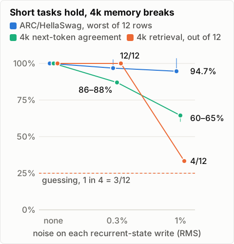
| Condition | 4k perplexity change | 4k next-token agreement | 4k retrieval |
|---|---|---|---|
| Clean / ideal | 0% | 100% | 12/12 |
| State write 0.3% | +4.2% to +10.2% | 85.6–87.8% | 12/12 |
| State write 1% | +90% to +140% | 60.4–65.0% | 4/12 |
| Combined case | +88% to +117% | 62.3–65.1% | 4/12 |
Ranges are across the three draws; retrieval ran on the first draw only. With four choices, guessing gets 3/12 on average, so 4/12 means the planted fact is effectively gone. My read is that the short benchmarks can't see this because their prompts are only tens to a few hundred tokens long. The recurrent state never has time to fill up with noise before the answer is scored.
The generations told a similar story in miniature. Every condition answered "46 + 27" correctly. The one-sentence explanation of why a metal spoon feels colder than a wooden one changed wording under noise, and at 1% it ran to the 32-token cap mid-sentence. Two prompts don't prove anything; they're there to catch a model that's falling apart.
Systematic errors behave differently
Random noise averages out a little. Error that pushes the same way every time doesn't. Multiplying the stored state by 1.001 on every write raised 4k perplexity by 73%. Multiplying it by 0.999 instead lowered perplexity by 3.7%, but still shifted the output distribution (mean KL 0.041), because it amounts to making the model forget faster than it was trained to. A gain that drifts by 1e-8 per token on top of the combined case moved 4k perplexity from +117% to +122% without changing any short-task score. For hardware, that suggests calibration and drift matter at least as much as the random noise floor on any stored state that gets rewritten.
What it cost
Each run rented one RTX 3090 with a $0.30/hour price cap and a 90-minute wall-clock limit. The runner uploads a hashed snapshot of the source, streams each finished result file back with its checksum as soon as it's written (so a host that dies mid-run still leaves evidence), then destroys the rental and checks that it's actually gone. The frozen 256-item run cost about 23 cents. The big exploratory sweep was 88 scored conditions in about 88 minutes for 27 cents. I wrote up renting GPUs this way for a fine-tuning project earlier, and the same failure modes showed up here. The frozen run hit its time limit during the very last 4k context, so one drift diagnostic is missing.
The protocol also included a second track: noise-aware fine-tuning, training small low-rank weight updates with the noisy state in the loop, to see how much of the loss could be trained away. Both permitted attempts and a separately registered extra attempt failed before training started (one lost SSH during setup, two never finished booting). Under the rules those slots stay empty. So I don't know yet whether fine-tuning recovers the long-context loss, and I'd rather report that than a result from a recipe I tweaked after seeing the first scores.
What I took from it
- Most of an inference path tolerates percent-level noise. Weights, projections, activations and especially the once-written KV cache handled 1% with almost no measurable effect, and several handled 10%.
- Anything rewritten every token is the hard part. In a hybrid model, that's the recurrent state, and 1% per write was already too much for long context. 0.3% looked fine on everything I measured, but that's 12 retrieval questions on one draw.
- Short benchmarks are the wrong test for memory. If I'd only run ARC and HellaSwag I would have concluded 1% was roughly fine.
- Digitizing doesn't automatically fix it. An ADC (analog-to-digital converter) on every state write would stop errors from piling up in storage, but it can't undo error that's already in the value it converts, and here it would have to handle 4.7 million values per token.
- Freeze the protocol before the expensive run. The cheap exploratory screens were useful for deciding where to look, and misleading as evidence.
Caveats
This is one small model, 256 items per task, three noise draws and 12 retrieval questions. The noise is a diagnostic unit, relative to each group's own signal, not a model of any real device. Error inside nonlinear functions, finite range, correlated noise across a device and read-back damage are all left out. Larger models, other architectures and pure-attention models may behave differently, and since a pure-attention model has no recurrent state, the headline finding may simply not apply to it. The KV cache tolerance results come from the exploratory screen, not the frozen run.